how to find the length of a curve

6.four: Arc Length of a Bend and Surface Area

1. Last updated

2. Save equally PDF

Page ID

2522

Learning Objectives

• Determine the length of a curve, \(y=f(x)\), between ii points.
• Make up one's mind the length of a curve, \(ten=thou(y)\), between two points.
• Observe the surface expanse of a solid of revolution.

In this section, nosotros utilize definite integrals to observe the arc length of a bend. We can think of arc length as the distance you would travel if you were walking along the path of the curve. Many real-world applications involve arc length. If a rocket is launched along a parabolic path, nosotros might want to know how far the rocket travels. Or, if a curve on a map represents a route, we might want to know how far we have to drive to achieve our destination.

Nosotros brainstorm by computing the arc length of curves defined as functions of \( x\), then nosotros examine the same process for curves defined as functions of \( y\). (The process is identical, with the roles of \( x\) and \( y\) reversed.) The techniques we use to notice arc length tin can be extended to notice the expanse of a surface of revolution, and we close the department with an exam of this concept.

Arc Length of the Curve y = f(x)

In previous applications of integration, nosotros required the office \( f(x)\) to be integrable, or at most continuous. Nevertheless, for calculating arc length we take a more stringent requirement for \( f(x)\). Here, we crave \( f(x)\) to be differentiable, and furthermore we crave its derivative, \( f′(x),\) to be continuous. Functions like this, which have continuous derivatives, are called smoothen. (This property comes upwardly again in subsequently capacity.)

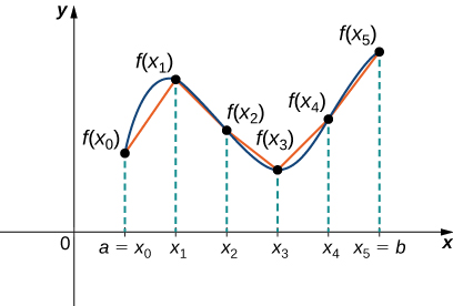
Let \( f(x)\) exist a smooth function defined over \( [a,b]\). We want to summate the length of the curve from the point \( (a,f(a))\) to the bespeak \( (b,f(b))\). We start past using line segments to approximate the length of the curve. For \( i=0,1,2,…,due north\), permit \( P={x_i}\) be a regular segmentation of \( [a,b]\). Then, for \( i=1,2,…,n\), construct a line segment from the point \( (x_{i−one},f(x_{i−one}))\) to the point \( (x_i,f(x_i))\). Although it might seem logical to utilise either horizontal or vertical line segments, we want our line segments to approximate the curve as closely equally possible. Figure \(\PageIndex{1}\) depicts this construct for \( due north=five\).

Effigy \(\PageIndex{1}\): Nosotros can judge the length of a bend by adding line segments.

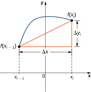
To help us find the length of each line segment, we look at the change in vertical distance as well as the alter in horizontal distance over each interval. Considering we have used a regular partition, the change in horizontal altitude over each interval is given by \( Δx\). The change in vertical altitude varies from interval to interval, though, and so we use \( Δy_i=f(x_i)−f(x_{i−1})\) to correspond the alter in vertical distance over the interval \( [x_{i−1},x_i]\), equally shown in Effigy \(\PageIndex{ii}\). Annotation that some (or all) \( Δy_i\) may exist negative.

Effigy \(\PageIndex{ii}\): A representative line segment approximates the curve over the interval \( [x_{i−i},x_i].\)

By the Pythagorean theorem, the length of the line segment is

\[ \sqrt{(Δx)^2+(Δy_i)^2}. \nonumber \]

We can also write this every bit

\[ Δx\sqrt{i+((Δy_i)/(Δx))^2}. \nonumber\]

Now, by the Hateful Value Theorem, in that location is a point \( 10^∗_i∈[x_{i−1},x_i]\) such that \( f′(ten^∗_i)=(Δy_i)/(Δx)\). Then the length of the line segment is given by

\[ Δx\sqrt{1+[f′(x^∗_i)]^2}. \nonumber\]

Adding up the lengths of all the line segments, nosotros go

\[\text{Arc Length} ≈\sum_{i=1}^n\sqrt{1+[f′(x^∗_i)]^2}Δx.\nonumber \]

This is a Riemann sum. Taking the limit as \( due north→∞,\) we have

\[\begin{marshal*} \text{Arc Length} &=\lim_{n→∞}\sum_{i=1}^n\sqrt{i+[f′(x^∗_i)]^2}Δx \\[4pt] &=∫^b_a\sqrt{1+[f′(x)]^ii}dx.\cease{align*}\]

Nosotros summarize these findings in the post-obit theorem.

Arc Length for \( y = f(x)\)

Permit \( f(10)\) be a polish role over the interval \([a,b]\). And so the arc length of the portion of the graph of \( f(x)\) from the signal \( (a,f(a))\) to the point \( (b,f(b))\) is given by

\[\text{Arc Length}=∫^b_a\sqrt{1+[f′(ten)]^ii}\,dx.\]

Note that we are integrating an expression involving \( f′(x)\), then nosotros need to be sure \( f′(x)\) is integrable. This is why we require \( f(10)\) to be smooth. The following case shows how to apply the theorem.

Example \( \PageIndex{1}\): Calculating the Arc Length of a Part of x

Allow \( f(x)=2x^{3/2}\). Calculate the arc length of the graph of \( f(x)\) over the interval \( [0,ane]\). Round the answer to three decimal places.

Solution

We take \( f′(x)=3x^{1/2},\) so \( [f′(x)]^2=9x.\) And so, the arc length is

\[\begin{marshal*} \text{Arc Length} &=∫^b_a\sqrt{ane+[f′(x)]^2}dx \nonumber \\[4pt] &= ∫^1_0\sqrt{1+9x}dx. \nonumber \cease{marshal*}\]

Substitute \( u=1+9x.\) So, \( du=9dx.\) When \( x=0\), so \( u=one\), and when \( x=1\), so \( u=10\). Thus,

\[ \begin{marshal*} \text{Arc Length} &=∫^1_0\sqrt{one+9x}dx \\[4pt] =\dfrac{one}{9}∫^1_0\sqrt{1+9x}9dx \\[4pt] &= \dfrac{1}{ix}∫^{x}_1\sqrt{u}du \\[4pt] &=\dfrac{ane}{9}⋅\dfrac{2}{iii}u^{iii/two}∣^{10}_1 =\dfrac{2}{27}[x\sqrt{ten}−ane] \\[4pt] &≈2.268units. \end{align*}\]

Practise \(\PageIndex{1}\)

Let \(f(x)=(4/3)ten^{iii/ii}\). Calculate the arc length of the graph of \( f(ten)\) over the interval \( [0,1]\). Round the respond to three decimal places.

Hint

Employ the procedure from the previous example. Don't forget to change the limits of integration.

Answer

\[ \dfrac{1}{6}(v\sqrt{5}−1)≈i.697 \nonumber\]

Although it is overnice to have a formula for calculating arc length, this particular theorem tin can generate expressions that are difficult to integrate. We study some techniques for integration in Introduction to Techniques of Integration. In some cases, we may accept to apply a reckoner or figurer to approximate the value of the integral.

Example \( \PageIndex{2}\): Using a Computer or Calculator to Determine the Arc Length of a Role of x

Allow \( f(10)=x^2\). Summate the arc length of the graph of \( f(x)\) over the interval \( [1,3]\).

Solution

We have \( f′(x)=2x,\) so \( [f′(ten)]^2=4x^2.\) Then the arc length is given past

\[\brainstorm{align*} \text{Arc Length} &=∫^b_a\sqrt{one+[f′(10)]^2}\,dx \\[4pt] &=∫^3_1\sqrt{1+4x^2}\,dx. \end{align*}\]

Using a computer to gauge the value of this integral, nosotros go

\[ ∫^3_1\sqrt{one+4x^two}\,dx ≈ 8.26815. \nonumber\]

Do \(\PageIndex{2}\)

Let \( f(x)=\sin x\). Summate the arc length of the graph of \( f(10)\) over the interval \( [0,π]\). Use a computer or calculator to approximate the value of the integral.

Hint

Use the process from the previous case.

Answer

\[ \text{Arc Length} ≈ 3.8202\]

Arc Length of the Curve \(x = g(y)\)

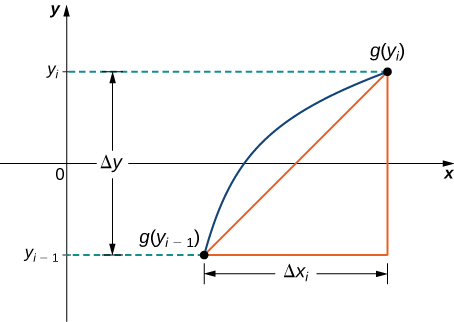
We have just seen how to approximate the length of a curve with line segments. If we desire to find the arc length of the graph of a function of \(y\), we tin repeat the same procedure, except we sectionalisation the y-axis instead of the x-axis. Figure \(\PageIndex{3}\) shows a representative line segment.

Figure \(\PageIndex{iii}\): A representative line segment over the interval \([y_{i−1},y_i].\)

So the length of the line segment is

\[\sqrt{(Δy)^2+(Δx_i)^two},\]

which can also exist written every bit

\[Δy\sqrt{ane+\left(\dfrac{Δx_i}{Δy}\right)^2}.\]

If nosotros now follow the same development nosotros did earlier, we get a formula for arc length of a role \(ten=g(y)\).

Arc Length for x = k(y)

Let \(k(y)\) exist a smooth function over an interval \([c,d]\). Then, the arc length of the graph of \(chiliad(y)\) from the indicate \((c,yard(c))\) to the point \((d,yard(d))\) is given by

\[\text{Arc Length}=∫^d_c\sqrt{1+[g′(y)]^2}dy.\]

Instance \(\PageIndex{iii}\): Calculating the Arc Length of a Role of \(y\)

Let \(g(y)=3y^3.\) Calculate the arc length of the graph of \(k(y)\) over the interval \([1,ii]\).

Solution

Nosotros have \(g′(y)=9y^2,\) and then \([g′(y)]^2=81y^four.\) And so the arc length is

\[\begin{align*} \text{Arc Length} &=∫^d_c\sqrt{1+[grand′(y)]^two}dy \\[4pt] &=∫^2_1\sqrt{one+81y^4}dy.\finish{align*}\]

Using a computer to approximate the value of this integral, we obtain

\[ ∫^2_1\sqrt{i+81y^4}dy≈21.0277.\nonumber\]

Do \(\PageIndex{iii}\)

Let \(g(y)=1/y\). Calculate the arc length of the graph of \(g(y)\) over the interval \([1,iv]\). Use a computer or calculator to gauge the value of the integral.

Hint

Apply the process from the previous example.

Answer

\[\text{Arc Length} =3.15018 \nonumber\]

Surface area of a Surface of Revolution

The concepts we used to find the arc length of a bend can be extended to detect the surface area of a surface of revolution. Surface area is the total surface area of the outer layer of an object. For objects such equally cubes or bricks, the surface area of the object is the sum of the areas of all of its faces. For curved surfaces, the situation is a little more complex. Let \(f(x)\) be a nonnegative smooth function over the interval \([a,b]\). We wish to find the area of the surface of revolution created past revolving the graph of \(y=f(x)\) around the \(x\)-axis as shown in the following figure.

Figure \(\PageIndex{iv}\): (a) A curve representing the function \(f(x)\). (b) The surface of revolution formed by revolving the graph of \(f(x)\) around the \(x-axis\).

Equally we have done many times before, we are going to division the interval \([a,b]\) and estimate the surface area past calculating the surface surface area of simpler shapes. We beginning by using line segments to judge the curve, as nosotros did earlier in this section. For \(i=0,i,2,…,n\), let \(P={x_i}\) be a regular sectionalization of \([a,b]\). And so, for \(i=1,two,…,n,\) construct a line segment from the point \((x_{i−i},f(x_{i−1}))\) to the point \((x_i,f(x_i))\). Now, revolve these line segments around the \(x\)-axis to generate an approximation of the surface of revolution as shown in the following figure.

Effigy \(\PageIndex{5}\): (a) Approximating \(f(x)\) with line segments. (b) The surface of revolution formed by revolving the line segments effectually the \(10-axis\).

Notice that when each line segment is revolved around the axis, information technology produces a ring. These bands are actually pieces of cones (think of an water ice cream cone with the pointy end cut off). A piece of a cone like this is chosen a frustum of a cone.

To notice the surface area of the band, we need to find the lateral surface area, \(Due south\), of the frustum (the area of just the slanted outside surface of the frustum, not including the areas of the top or lesser faces). Let \(r_1\) and \(r_2\) be the radii of the wide terminate and the narrow finish of the frustum, respectively, and allow \(l\) be the camber top of the frustum equally shown in the post-obit figure.

Figure \(\PageIndex{6}\): A frustum of a cone tin approximate a small part of surface expanse.

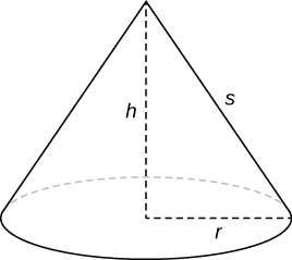
Nosotros know the lateral surface area of a cone is given past

\[\text{Lateral Surface Area } =πrs,\]

where \(r\) is the radius of the base of operations of the cone and \(s\) is the camber height (Figure \(\PageIndex{seven}\)).

Figure \(\PageIndex{7}\): The lateral surface area of the cone is given by \(πrs\).

Since a frustum can be thought of every bit a piece of a cone, the lateral surface area of the frustum is given by the lateral surface area of the whole cone less the lateral surface area of the smaller cone (the pointy tip) that was cutting off (Figure \(\PageIndex{8}\)).

Figure \(\PageIndex{eight}\): Computing the lateral surface area of a frustum of a cone.

The cross-sections of the small-scale cone and the big cone are similar triangles, so we see that

\[ \dfrac{r_2}{r_1}=\dfrac{s−50}{s}\]

Solving for \(s\), we go =southward−ls

\[\brainstorm{marshal*} \dfrac{r_2}{r_1} &=\dfrac{due south−l}{south} \\ r_2s &=r_1(s−50) \\ r_2s &=r_1s−r_1l \\ r_1l &=r_1s−r_2s \\ r_1l &=(r_1−r_2)s \\ \dfrac{r_1l}{r_1−r_2} =southward \stop{marshal*}\]

Then the lateral area (SA) of the frustum is

\[\begin{align*} S &= \text{(Lateral SA of large cone)}− \text{(Lateral SA of small cone)} \\[4pt] &=πr_1s−πr_2(southward−fifty) \\[4pt] &=πr_1(\dfrac{r_1l}{r_1−r_2})−πr_2(\dfrac{r_1l}{r_1−r_2−l}) \\[4pt] &=\dfrac{πr^2_1l}{r^1−r^2}−\dfrac{πr_1r_2l}{r_1−r_2}+πr_2l \\[4pt] &=\dfrac{πr^2_1l}{r_1−r_2}−\dfrac{πr_1r2_l}{r_1−r_2}+\dfrac{πr_2l(r_1−r_2)}{r_1−r_2} \\[4pt] &=\dfrac{πr^2_1}{lr_1−r_2}−\dfrac{πr_1r_2l}{r_1−r_2} + \dfrac{πr_1r_2l}{r_1−r_2}−\dfrac{πr^2_2l}{r_1−r_3} \\[4pt] &=\dfrac{π(r^2_1−r^2_2)l}{r_1−r_2}=\dfrac{π(r_1−r+ii)(r1+r2)l}{r_1−r_2} \\[4pt] &= π(r_1+r_2)fifty. \label{eq20} \finish{marshal*}\]

Permit's now use this formula to summate the surface surface area of each of the bands formed by revolving the line segments effectually the \(x-axis\). A representative band is shown in the following effigy.

Figure \(\PageIndex{9}\): A representative ring used for determining surface area.

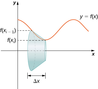
Annotation that the slant height of this frustum is just the length of the line segment used to generate it. So, applying the surface area formula, we have

\[\begin{align*} S &=π(r_1+r_2)50 \\ &=π(f(x_{i−1})+f(x_i))\sqrt{Δx^2+(Δyi)^2} \\ &=π(f(x_{i−1})+f(x_i))Δx\sqrt{1+(\dfrac{Δy_i}{Δx})^2} \end{align*}\]

Now, every bit we did in the development of the arc length formula, we apply the Hateful Value Theorem to select \(x^∗_i∈[x_{i−i},x_i]\) such that \(f′(x^∗_i)=(Δy_i)/Δx.\) This gives us

\[Due south=π(f(x_{i−1})+f(x_i))Δx\sqrt{1+(f′(x^∗_i))^2} \nonumber\]

Furthermore, since\(f(10)\) is continuous, by the Intermediate Value Theorem, there is a bespeak \(x^{**}_i∈[x_{i−1},x[i]\) such that \(f(ten^{**}_i)=(1/2)[f(xi−i)+f(11)],

then we get

\[S=2πf(x^{**}_i)Δx\sqrt{1+(f′(x^∗_i))^two}.\nonumber\]

Then the approximate surface surface area of the whole surface of revolution is given past

\[\text{Surface Expanse} ≈\sum_{i=ane}^n2πf(x^{**}_i)Δx\sqrt{1+(f′(10^∗_i))^two}.\nonumber\]

This almost looks like a Riemann sum, except we have functions evaluated at 2 different points, \(10^∗_i\) and \(x^{**}_{i}\), over the interval \([x_{i−i},x_i]\). Although we do not examine the details here, it turns out that because \(f(x)\) is smooth, if nosotros let n\(→∞\), the limit works the aforementioned as a Riemann sum even with the two different evaluation points. This makes sense intuitively. Both \(x^∗_i\) and 10^{**}_i\) are in the interval \([x_{i−1},x_i]\), so it makes sense that every bit \(n→∞\), both \(10^∗_i\) and \(10^{**}_i\) approach \(x\) Those of you who are interested in the details should consult an advanced calculus text.

Taking the limit every bit \(northward→∞,\) we get

\[ \brainstorm{align*} \text{Surface Area} &=\lim_{north→∞}\sum_{i=one}due north^2πf(x^{**}_i)Δx\sqrt{one+(f′(x^∗_i))^2} \\[4pt] &=∫^b_a(2πf(x)\sqrt{one+(f′(x))^two}) \finish{align*}\]

Equally with arc length, we tin conduct a like development for functions of \(y\) to get a formula for the surface area of surfaces of revolution about the \(y-centrality\). These findings are summarized in the following theorem.

Surface Area of a Surface of Revolution

Let \(f(ten)\) exist a nonnegative smoothen role over the interval \([a,b]\). Then, the surface area of the surface of revolution formed by revolving the graph of \(f(10)\) around the 10-axis is given by

\[\text{Area}=∫^b_a(2πf(x)\sqrt{1+(f′(x))^ii})dx\]

Similarly, let \(g(y)\) be a nonnegative smooth function over the interval \([c,d]\). Then, the surface surface area of the surface of revolution formed by revolving the graph of \(grand(y)\) around the \(y-centrality\) is given by

\[\text{Surface Area}=∫^d_c(2πg(y)\sqrt{i+(yard′(y))^2}dy\]

Example \(\PageIndex{iv}\): Calculating the Surface Area of a Surface of Revolution 1.

Let \(f(x)=\sqrt{x}\) over the interval \([1,4]\). Observe the surface area of the surface generated by revolving the graph of \(f(x)\) around the \(x\)-centrality. Round the reply to three decimal places.

Solution

The graph of \(f(x)\) and the surface of rotation are shown in Effigy \(\PageIndex{10}\).

Figure \(\PageIndex{10}\): (a) The graph of \(f(x)\). (b) The surface of revolution.

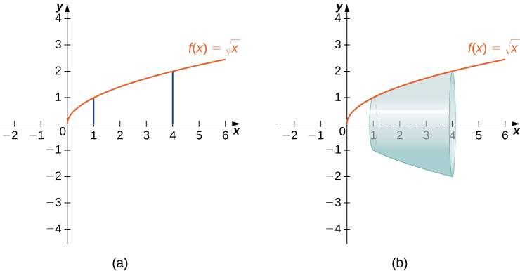
Nosotros have \(f(ten)=\sqrt{10}\). Then, \(f′(x)=ane/(2\sqrt{ten})\) and \((f′(x))^2=1/(4x).\) So,

\[\begin{align*} \text{Surface Expanse} &=∫^b_a(2πf(ten)\sqrt{1+(f′(ten))^2}dx \\[4pt] &=∫^4_1(\sqrt{2π\sqrt{x}1+\dfrac{ane}{4x}})dx \\[4pt] &=∫^4_1(2π\sqrt{x+14}dx. \end{align*}\]

Let \(u=x+1/iv.\) Then, \(du=dx\). When \(x=i, u=5/4\), and when \(x=4, u=17/four.\) This gives u.s.

\[\begin{align*} ∫^1_0(2π\sqrt{x+\dfrac{1}{iv}})dx &= ∫^{17/4}_{5/4}2π\sqrt{u}du \\[4pt] &= 2π\left[\dfrac{two}{3}u^{3/ii}\right]∣^{17/4}_{5/iv} \\[4pt] &=\dfrac{π}{6}[17\sqrt{17}−five\sqrt{5}]≈30.846 \end{align*}\]

Exercise \(\PageIndex{4}\)

Permit \( f(10)=\sqrt{1−x}\) over the interval \( [0,1/2]\). Discover the area of the surface generated past revolving the graph of \( f(x)\) around the \(x\)-centrality. Round the reply to three decimal places.

Hint

Apply the procedure from the previous example.

Answer

\[ \dfrac{π}{6}(5\sqrt{5}−three\sqrt{3})≈3.133\]

Example \( \PageIndex{5}\): Calculating the Surface Area of a Surface of Revolution 2

Allow \( f(ten)=y=\dfrac[3]{3x}\). Consider the portion of the curve where \( 0≤y≤ii\). Find the surface surface area of the surface generated by revolving the graph of \( f(10)\) around the \( y\)-axis.

Solution

Notice that we are revolving the bend around the \( y\)-axis, and the interval is in terms of \( y\), and then we want to rewrite the function as a function of \( y\). We get \( x=g(y)=(1/3)y^3\). The graph of \( grand(y)\) and the surface of rotation are shown in the following figure.

Effigy \(\PageIndex{11}\): (a) The graph of \( g(y)\). (b) The surface of revolution.

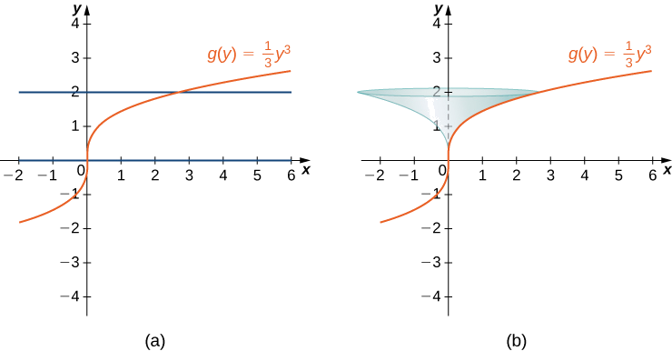
We have \( g(y)=(1/3)y^3\), so \( chiliad′(y)=y^2\) and \( (g′(y))^2=y^iv\). And so

\[\brainstorm{align*} \text{Surface Expanse} &=∫^d_c(2πg(y)\sqrt{1+(g′(y))^2})dy \\[4pt] &=∫^2_0(2π(\dfrac{1}{3}y^3)\sqrt{one+y^4})dy \\[4pt] &=\dfrac{2π}{iii}∫^2_0(y^3\sqrt{1+y^4})dy. \end{marshal*}\]

Allow \( u=y^four+1.\) And so \( du=4y^3dy\). When \( y=0, u=1\), and when \( y=2, u=17.\) Then

\[\brainstorm{marshal*} \dfrac{2π}{3}∫^2_0(y^3\sqrt{1+y^4})dy &=\dfrac{2π}{3}∫^{17}_1\dfrac{1}{4}\sqrt{u}du \\[4pt] &=\dfrac{π}{6}[\dfrac{two}{iii}u^{3/2}]∣^{17}_1=\dfrac{π}{9}[(17)^{3/ii}−one]≈24.118. \end{align*}\]

Practise \(\PageIndex{5}\)

Let \( g(y)=\sqrt{9−y^2}\) over the interval \( y∈[0,2]\). Find the surface area of the surface generated past revolving the graph of \( chiliad(y)\) around the \( y\)-axis.

Hint

Employ the process from the previous example.

Answer

\( 12π\)

Key Concepts

• The arc length of a bend tin can exist calculated using a definite integral.
• The arc length is start approximated using line segments, which generates a Riemann sum. Taking a limit and then gives us the definite integral formula. The same procedure can be practical to functions of \( y\).
• The concepts used to calculate the arc length can exist generalized to discover the surface area of a surface of revolution.
• The integrals generated past both the arc length and surface expanse formulas are oftentimes hard to evaluate. It may be necessary to use a computer or calculator to guess the values of the integrals.

Primal Equations

• Arc Length of a Office of x

Arc Length \( =∫^b_a\sqrt{1+[f′(x)]^two}dx\)

• Arc Length of a Function of y

Arc Length \( =∫^d_c\sqrt{1+[grand′(y)]^two}dy\)

• Surface Expanse of a Function of x

Surface Area \( =∫^b_a(2πf(ten)\sqrt{i+(f′(x))^2})dx\)

Glossary

arc length

the arc length of a bend can be thought of equally the altitude a person would travel along the path of the curve

frustum

a portion of a cone; a frustum is synthetic by cutting the cone with a airplane parallel to the base

surface surface area

the surface area of a solid is the total area of the outer layer of the object; for objects such as cubes or bricks, the surface area of the object is the sum of the areas of all of its faces

Source: https://math.libretexts.org/Bookshelves/Calculus/Book%3A_Calculus_(OpenStax)/06%3A_Applications_of_Integration/6.4%3A_Arc_Length_of_a_Curve_and_Surface_Area

Posted by: jonesaffeekly.blogspot.com

Share this post